The EarthScope-operated data systems of the NSF GAGE and SAGE Facilities are migrating to cloud services. To learn more about this effort and find resources, visit earthscope.org/data/cloud

The digital and print versions of a book contain the same information, but that doesn’t mean your access to that information is exactly the same. For example, you could sate an odd curiosity and find out how many times the word “orchard” appears with a few keystrokes and a few seconds of waiting with the digital version. Using the print version to answer this question would be an entirely different kind of endeavor.

Moving the NSF GAGE and SAGE data archives to the cloud—and then optimizing them for cloud operations—is all about making them as little like that printed book as possible. We want scientific inquiries to face as few speedbumps as possible, enabling you to do more with less time invested. This is a key part of our ARCO vision: Analysis-Ready, Cloud-Optimized. Let’s talk a little about the way we’re structuring data storage to help make that happen.

I object

Moving to cloud data storage means entering the world of object storage. On your own computer, you’re accustomed to interacting with a file storage system. This organizes your files in a hierarchical folder structure. To find and access a file, you need to know the nested folder path to it, in addition to the name you’ve given it.

This has loads of benefits for keeping things tidy—if you maintain a tidy structure instead of naming everything “project_new”, “project_new_new”, and “project_new_new_2”—but file storage comes with logistical ceilings. As the number of files and folders grows, the computational costs of search and access also grow.

Cloud storage systems instead opt for object storage, which has no hierarchy. Instead, each file or chunk of data forms an object, with attached metadata and a unique identifier that serves as the simple locator by which it can be accessed. In this system, there is no folder structure to constantly dig into and out of, and there is fundamentally no limit on the scale this can expand to. There is just one big pool of objects. This is ideal for ARCO because it allows us to create a distributed and redundant storage system, where data is replicated across multiple servers and locations for increased reliability and durability. And since cloud storage costs are typically based on usage, this approach is inherently cost-effective, especially for data that are written once and then periodically retrieved.

Using object storage doesn’t automatically mean you’re ready to drive machine learning processing at breakneck speed, however. It’s easy to imagine launching all your data into one towering pile of objects without a good way to quickly fetch just the files you want to answer a specific question. But an object storage system allows for deep optimization of cloud computing, with a large number of compute nodes quickly and efficiently accessing data simultaneously.

We can rebuild it

One way we’re building in that optimization is through the data format. For many types of data, we’re building around TileDB—a library that efficiently manages large-scale array data. TileDB provides a data array structure and database-like engine that, when combined with object storage, is a great fit for large scale analysis for several reasons.

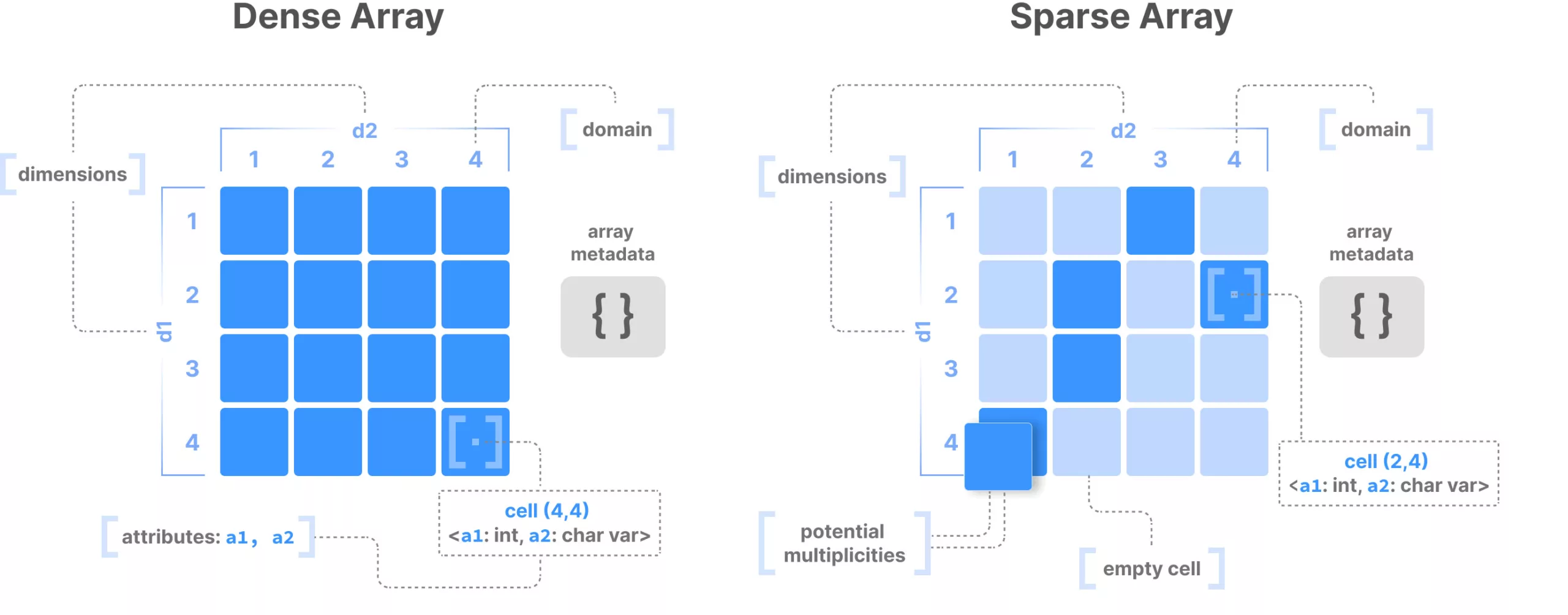
For one, it allows for sparse arrays, meaning we don’t need to write null values (which increase storage size and make for inefficient processing) in empty cells. With TileDB, the empty cells simply don’t exist at all. These arrays can have any number of dimensions, and data can efficiently be queried from the array based on one or more dimensions. This includes versioning—if a cell value is rewritten, each version is retained and can be accessed by specifying a point in time. And TileDB supports parallelized read/write activity, so powerful multi-threaded compute resources won’t hit a bottleneck. The metadata for these datasets are handled by separate relational databases that are being carefully designed to make it as easy as possible to query up the data you’re after—wherever it is stored.

The idea is to use a standardized, efficient storage array that can serve data in any format you need. You can pull your queried data directly into a data frame that is ready for processing, or you can use tools we’re creating to pull that data into a familiar file format to work with, instead. There is much more flexibility in this approach.

For example, GNSS data users are well acquainted with the humble RINEX file, an ASCII-formatted collection of observations and metadata produced for each day. Because the data can go through several rounds of corrections, and users may wish to work with datasets at different sampling rates, we end up with multiple copies of RINEX files for a given instrument each day—duplicated yet again to store in RINEX 2, 3, and 4 formats. And working with downloaded RINEX data requires first reading it out of the ASCII files (spanning multiple daily files) and into a data frame.

In our TileDB implementation for GNSS data, we use a single data array per station. When new observations or corrected positions become available, they are appended as new versions of each cell in the array. This approach allows seamless access to both rapid positions and corrected positions from the same array.

The dimensions of this array include the time of each observation and the corresponding constellation, satellite, and observation codes (like frequency). And within those dimensions we can store the measured values of range, phase, signal-to-noise, and so on. Because only some satellites are visible at a given time, almost two-thirds of these cells are empty—but as a sparse array, TileDB does not require us to store these null values.

This array can then be queried over one or more dimensions to limit your searches for only the specific values you’re interested in, whether that’s the signal-to-noise ratio of a single satellite over the course of a certain day, or all observations at a 1 Hz sample rate for six months.

For a quick example, we’ll go back to a demo we’ve referenced previously and compare two pieces of Python code that both allow us to calculate daily means of the signal-to-noise ratio on the L1C signal for GPS constellation satellites at a station in Utah. (Note that these aren’t complete scripts and won’t run as-is. We’ve left out the rest to focus on how these two methods differ.)

Here’s what that looks like when you download multiple daily RINEX files and create a data frame containing the values we’re after—with the help of the GeoRinex package.

start_t = time.time()
for doy in np.arange(1,10):
    #download
    url='https://gage-data.earthscope.org/archive/gnss/rinex/obs/2024/%03d/p057%03d0.24d.Z' %(doy,doy)
    print('downloading: ', url)
    get_es_file(url, 'rinex_data')
   
    #process
    fn='rinex_data/p057%03d0.24d.Z' %doy
    # Use Georinex to convert Rinex _> Xarray Dataframe
    obs = gr.load(fn, use='G', meas=['S1'])
    g=obs['S1'].mean().values
    snr_li+=[g]
    date_li+=[datetime(year, 1, 1) + timedelta(days=int(doy - 1))]
    #delete the file
    os.remove(fn)
   
end_t = time.time()
dl_time=end_t-start_t


snr_rnx=np.mean(snr_li)

Now let’s try that while accessing data stored in TileDB via (an early beta version of) our API, and similarly calculate daily means. (The unique identifier for this station’s dataset, also retrieved via API, is here stored in “uri”.)

%%time
start_t = time.time()


snr_li=[]
date_li=[]
for doy in np.arange(1,51):
    start=datetime(year, 1, 1) + timedelta(days=int(doy - 1))
    date_li+=[start]
    end=start+timedelta(days=1)
    start=unix_time_millis(start)
    end=unix_time_millis(end)
 
    with tiledb.open(uri,mode="r", config=tdb_config,) as A:
        df=A.df[slice(int(start), int(end)),constell,:,obs_code]['snr']
        snr_li+=[df.mean()]
       
for_loop=np.nanmean(np.array(snr_li))


end_t = time.time()
for_loop_t=end_t - start_t

Running this in our notebook hub, the first method took about 30 seconds to gather data for 9 days. The second method gathered 50 days in that same amount of time.

Rather than making intermediate file copies and using a helper package to read in data from those copies, there’s a direct data access pathway with TileDB. The model can change from “grab and convert to something useful” to just “grab what’s useful”.

Welcome to the Matrix (of shelves)

Optimizing the data archive for cloud computing means more than just changing storage format. The data—and metadata—must be organized thoughtfully, and the systems that facilitate access have to be well designed. The end goal is an extremely tidy and efficient data warehouse where the data you need can be retrieved from the shelves as effortlessly and quickly as possible, even as many other users are also retrieving data and deliveries of new data arrive every second.

That’s what will enable researchers to throw far more compute resources at a question than they could before—and will make the orchestration of those compute resources less complex.

We’re currently busy developing all these warehouse systems. Beyond GNSS data (which are already streaming into TileDB arrays), we are also planning to migrate data from borehole strainmeters, active source PH5 experiments, and DAS systems into TileDB storage. However, seismic miniSEED data storage has much less to gain from conversion—it already works well in object storage with widely available tools—and is currently slated to continue in that format.

As the archives increasingly serve analysis-ready, cloud-optimized data, we’re looking forward to finding out what new things the research community can do—which we hope will  be more impressive than counting the 21 occurrences of the word “orchard” in The Grapes of Wrath.

---

P.S. Let’s talk at AGU

The EarthScope-operated data systems of the NSF GAGE and SAGE Facilities continue their migration to the cloud—a transformative effort enhancing geophysical research through scalable, data-adjacent computing resources. At this year’s AGU meeting, there are several opportunities to learn more about the progress and future of this effort. Seven presentations will showcase different facets of this transition, from introducing tools like the GeoLab JupyterHub to sharing advancements in data accessibility, identity management, and infrastructure modernization.

These presentations highlight the collaborative work across the geophysical community, focusing on empowering researchers with tools that facilitate equitable access to cloud resources, seamless data workflows, and reproducible research. Topics range from technical deep dives into new data systems to forward-looking discussions about integrating cloud computing with workforce development and interdisciplinary research.

We invite attendees to explore these presentations to gain insights into EarthScope’s efforts to modernize data facilities and foster a more inclusive and collaborative scientific ecosystem. Whether you’re interested in technical infrastructure, community-focused training initiatives, or new approaches to data management, join us and be part of the conversation!

Cloud On-Ramp Presentations

• Broadening Access to Magnetotellurics Through Specialized Short Courses
• Introducing GeoLab – An EarthScope JupyterHub for Enabling Collaborative Cloud-Native Geophysical Data Analysis and Skill Development Workshops
• Seamless Authentication Capabilities for EarthScope Geophysical Data Services
• Initial Efforts Towards Archiving and Support for GNSS-A Data Processing in the EarthScope Cloud Platform
• EarthScope’s On-Ramp into Cloud Computing
• Towards the next generation of federated seismological data services
• EarthScope’s Cloud Migration: Building Analysis-Ready Geophysical Data Interfaces