


One of the major benefits of migrating our data archives to a cloud-native architecture is that we can offer new ways to interact with data. We’re building the systems that enable you to do that, including a Software Development Kit (SDK) that already has a lot to offer for GNSS data users.
GNSS interferometric reflectometry (GNSS-IR) provides a useful example because preparing its inputs can require substantially more code and file handling than the core analysis itself.
The technique
A GNSS antenna receives not only the signal arriving directly from a satellite but also a signal reflected off the surfaces around the antenna. The two arrive slightly out of phase, interfere, and leave a signature in the recorded signal-to-noise ratio (SNR): as a satellite rises or sets, the SNR oscillates.
The frequency of that oscillation depends on the reflector height and the distance from the antenna to the reflecting surface. Recover the frequency and you can recover the height of the reflecting surface. Track it over time and you’re measuring changes in the surface itself: snow accumulating and melting, water levels rising and falling, changes in soil moisture and vegetation. With this method, a geodetic station built to measure crustal motion can be an environmental sensor as well, using data it has been recording all along.
The analysis is compact. For each satellite, you need two things: the SNR on a chosen signal, and where that satellite was in the sky (i.e., its elevation and azimuth at every time epoch). The analysis involves detrending the SNR against the sine of the elevation angle, running a Lomb-Scargle periodogram over frequencies corresponding to a grid of candidate reflector heights, and identifying which reflector height corresponds to the strongest peak.
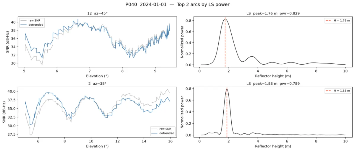
When data preparation dominates the workflow
In the traditional file-based workflow, assembling those two inputs takes several steps before any analysis begins.
GNSS observations have traditionally been distributed as RINEX files with one file per station per UTC day. If you want a season of data from one station, that’s on the order of ninety files to fetch, and proportionally more for a network. Each file can contain observations from every constellation, satellite, signal, and observable recorded during that session, including pseudorange, carrier phase, and SNR. Reflectometry needs only a narrow subset: SNR for a selected signal, together with the identifiers and timestamps needed to match each observation to its satellite geometry. Most of the downloaded RINEX is unused.
The second input, satellite elevation and azimuth, is not directly provided in RINEX observation files. You must obtain navigation or precise-orbit products separately and compute the geometry relative to the station’s coordinates. Add parsing, decimation to a common sampling interval, and merging the two streams, and you have a pipeline to build and maintain before you’ve computed a single reflector height.
The same workflow using the EarthScope SDK
Here’s the same setup, expressed as requests rather than files. Authentication happens once through the EarthScope CLI, or when you log into GeoLab, and then you describe what you want.
First, the observations:
obs = client.data.gnss_observations(
start_datetime=start,
end_datetime=end,
station_name=STATION,
system=["G"],
field="snr",
obs_code="1C",
sample_interval=dt.timedelta(seconds=15),
session_name="A",
).fetch().to_pandas()
The short codes follow RINEX conventions: G selects GPS satellites, while R, E, and C select GLONASS, Galileo, and BeiDou, and 1C is the L1 C/A signal. session_name identifies which data session at the station to draw from.
Every argument after the time range narrows the request, and the narrowing happens server-side. You aren’t downloading a day’s worth of everything and filtering locally; you’re asking for one constellation, one signal, one measurement column, at one sampling interval, and that is what crosses the network. The requested time range also does not have to align with UTC day boundaries the way RINEX does, so an arc that is calculated from multiple days of data doesn’t require stitching files together.
Second, the geometry:
eph = client.data.gnss_ephemeris_positions(
start_datetime=start,
end_datetime=end,
system=["G"],
field=["elevation", "azimuth"],
reference_point=ref_pt,
elevation_filter=FloatFilter(min=3.0),
sample_interval=dt.timedelta(seconds=15),
).fetch().to_pandas()
This request replaces the need to obtain and process orbit files. Pass the geodetic coordinate (`reference_point`) for your station, and elevation and azimuth are returned already computed with respect to that point, on the same sampling interval as the observations. The elevation_filter removes satellites below the lower cutoff before the data is sent, reducing the number of rows that must be transferred. The upper limit of the reflectometry window can then be applied during arc processing.
Because the results arrive as Apache Arrow tables, users do not have to parse RINEX text files before loading the data into a DataFrame.
What remains is a simple join between the observation and geometry tables. With data processing completed, the science can begin: split each satellite’s track into rising and setting arcs, remove a low-order polynomial trend from the SNR, and run the periodogram. That code is short, and it’s the part specific to reflectometry.
Scaling up
A targeted request for a single day can fit comfortably in memory, but a season of data across a network may not. The SDK handles that with query plans. For larger requests, you can leave off .fetch() to create a query plan. The plan can then be grouped by day, by station, or according to a custom strategy and processed one group at a time. The full request never has to fit in memory at once.
The upshot
Nothing here changes the underlying physics or reflector-height estimator. What changes is the balance between setup and analysis. The SDK enables requesting the specific inputs the workflow requires: SNR observations for a selected signal and constellation, at a chosen sampling interval, together with satellite geometry computed for the station. The results arrive in analysis-ready tables, eliminating local RINEX parsing and reducing both network transfer and memory use. This removes much of the tedious housekeeping that once stood between a research question and a result.
This same pattern generalizes. Reflectometry is a convenient example because of the specific analytic requirements, but any workflow that needs a narrow slice of a wide archive benefits in the same way.
A complete, runnable notebook for the workflow described here is available on GitHub. For instructions on installation and authentication, guidance on query plans, and additional examples across our data products, see the SDK documentation.