In addition to using GPS stations to measure ground movement associated with earthquakes, there have recently been efforts to also measure ionospheric signals caused by earthquakes and tsunamis. In order to extract as much information as possible from that kind of data, we need to understand the patterns of these ionospheric signals in great detail. In a recent paper published in Geophysical Research Letters, a team led by Pavel Inchin used the 2016 magnitude 7.8 Kaikoura earthquake to see what we could learn from testing the data against ionospheric simulations.

Because the ionosophere affects signals from navigation satellites—an important source of error to correct for more accurate position measurements—GPS stations (more generally known as GNSS) can also be used to measure ionospheric activity. Specifically, they can measure the “total electron content along the path between the station and each satellite in the sky. The ionosphere is defined by ionized gas—that is, charged gas molecules—so anything that excites or disturbs the ionosphere causes a change in the total electron content in that area.

While space weather is a familiar cause of ionospheric activity, movements of the lower atmosphere can also lead to detectable patterns of ionospheric activity. Just as a swimming fish can cause ripples in the surface of a pond, disturbing the ionosphere from below can make waves.

Volcanic eruptions, earthquakes, and tsunamis are all capable of producing these ionospheric waves, which can be observed in real time by GPS stations. But to make those observations useful in the moment, we need to be able to recognize the patterns of those waves. In this study, the research team used a model of the atmosphere to simulate the disturbance caused by the Kaikoura earthquake. Comparing that to GPS measurements of ionospheric total electron content can show how well they captured the big picture pattern.

For an apples-to-apples comparison, they tried to match the GPS measurements exactly. That means putting each station at the correct location in the model, and each satellite at its position in the sky during each measurement, so the total electron content along the line between them can be calculated.

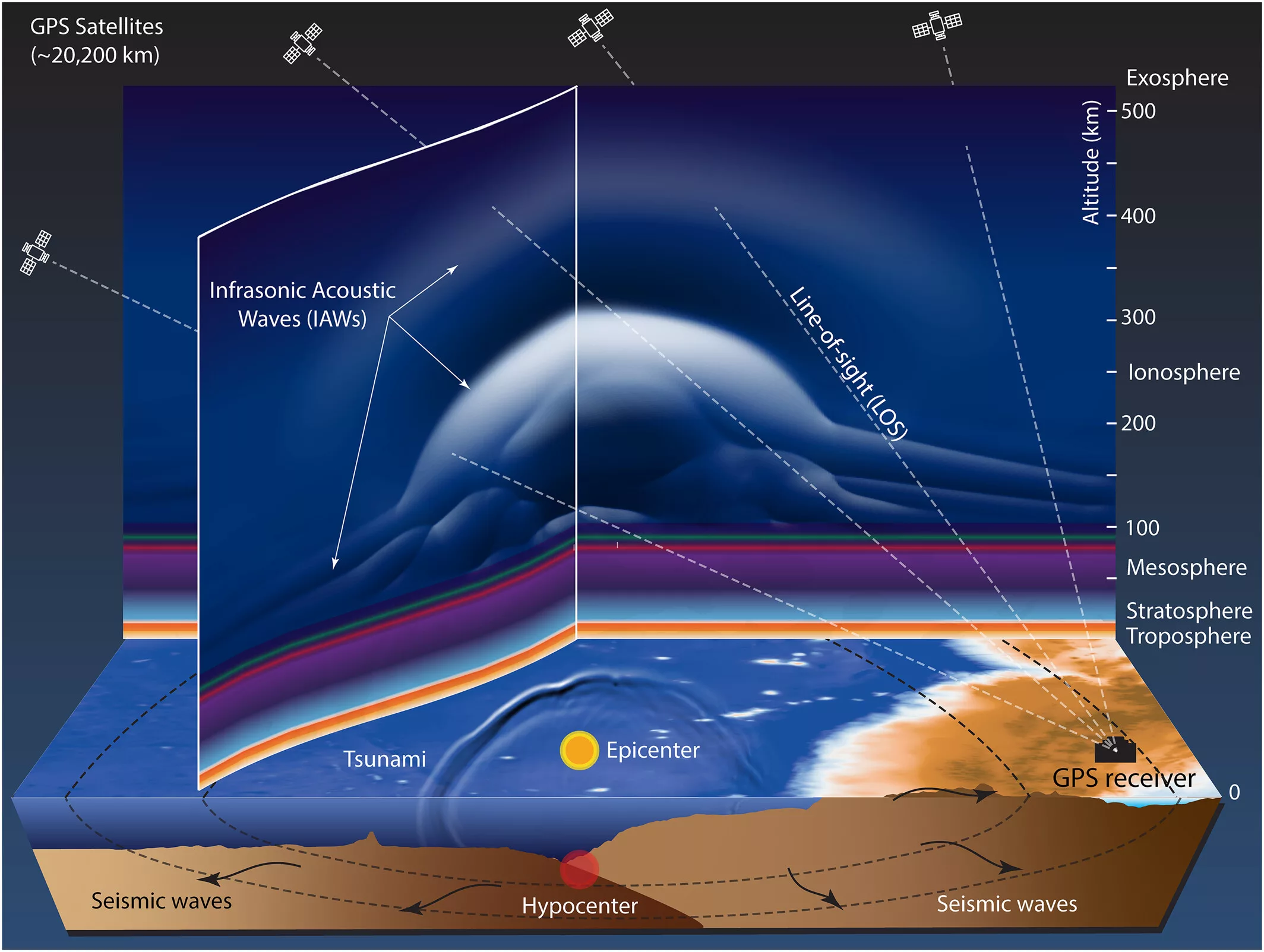
Using a previously published estimate of exactly how the fault moved during Kaikoura earthquake, the model simulated the way the surface seismic waves propagated up into the atmosphere and eventually disturbed the ionosphere. The result was waves of fluctuating total electron content moving north and south from the epicenter.

The GPS station measurements in the model match quite closely to the real-world GPS measurements—with a couple interesting exceptions. For one, the simulated fluctuation north of the epicenter was smaller than what the real-world data showed. And the simulated fluctuation to the east showed up about 20 seconds sooner than in the real-world data. This could be due to inaccuracies in the solid Earth part of the simulation, or perhaps to a missing local detail in the atmospheric behavior.

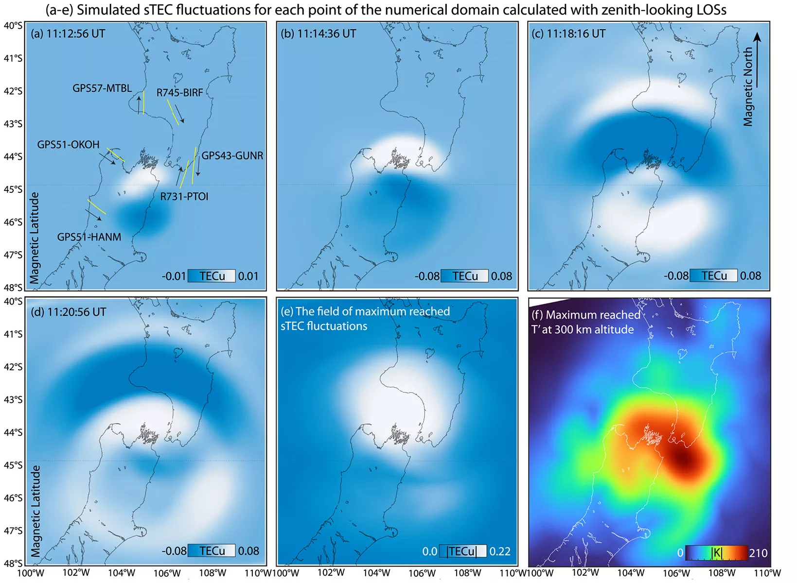
One more interesting finding is that a few of the measurements weren’t able to detect the initial appearance of an ionospheric wave for reasons of simple geometry. When the line between the GPS station and the satellite goes through both the peak and trough of a wave, the two cancel out. This means that a signal isn’t recognizable until the wave progresses a bit more—a useful consideration when analyzing all the data to detect or reconstruct an earthquake.

On the flip side, the researchers say that the ionospheric observations were detailed enough that they could be used to test and improve estimates of fault movement. The available seismic and geodetic data are used as inputs when calculating exactly where patches of the fault moved, and by how much. Adding another type of data means you can potentially fill in a gap and improve those calculations.

Putting more tools in the toolkit is always a good thing—and with research like this, we can figure out how best to put those tools to work.