

Earth’s surface is blanketed in places by the sands, muds, cobbles, and boulders of sediment. In basins, these layers may be quite thick — on the order of kilometers — whereas elsewhere, sediment may form a thin veneer. Sediment thickness can affect how strong shaking from an earthquake might be; its measurement can be crucial for seismic studies.
Despite the importance of where sediment is, and isn’t, no single map of sediment thickness across the conterminous U.S. exists that uses a consistent method — until now. In a new paper published in Seismological Research Letters, a team of scientists led by Augustin Marignier, a postdoctoral research at the Australian National University (now at the University of Oxford), used the NSF-funded Transportable Array data to extract information from the interface between sediment and the basement rock upon which it rests.
With this information, the team produced two maps of sediment thickness: one using an empirical borehole relation, and the other using the mean velocity in the upper 5 kilometers of an existing tomographic model produced via Transportable Array data. They found that the second map is an excellent first-order estimate of sediment thickness across the lower 48 states of the U.S.
Why thickness matters
Sediment thickness pertains to seismic studies in a number of ways.
When it comes to seismic hazard assessment, thick sediments can amplify seismic waves from an earthquake, which means more shaking. If thickness is unknown or underestimated, predictions of expected shaking might be too low. Basins full of sediment can also trap seismic waves, causing the waves to reverberate, resulting in longer shaking duration. The 2018 update to the U.S. National Seismic Hazard Model was the first to include basin depth, although only for the western U.S.
Studies of changes in seismic wave speed may also need to incorporate sediment thickness. Sediments slow seismic waves. If the thickness of a “slow” section isn’t properly characterized, regional tomographic images can be incorrect.
Numerous studies have looked at the thickness of sediments in specific basins across the U.S.
However, mapping efforts across the continent typically use specific and varied methods. Currently, the most commonly used map of sediment thickness for the U.S. is based on a compilation of hydrocarbon exploration studies. Published in 2010, this map is more detailed in certain regions because it is built via regional and local studies. However, certain spots lack information, and that deficit has propagated into the compilation.
USArray’s Transportable Array
In 2004, the Transportable Array, part of the USArray project, began its eastward march across the contiguous U.S. Each station operated for about two years, initially on the West Coast, before leapfrogging east. By 2013, seismic data from the lower 48 states was logged, and the project moved to Alaska.
Facilitated by this immense dataset, the seismic structure of the U.S. has been extensively studied. Much work has focused on one of the most famous of Earth’s seismic boundaries, the Mohorovičić discontinuity. The “Moho,” as it is often called, marks a dramatic change in seismic wave velocity as crust meets mantle.
But other seismic discontinuities exist, some of which may be marked by more subtle changes in velocity. The boundary between sediment and basement in particular tends to be blurred. Sometimes, models simply include the shallow sediment layer as part of Earth’s crust.
How to measure sediment thickness
There are two typical ways to determine sedimentary thickness. One method is to find specific shear wave velocity contours from tomographic models — either the depth of the 1 kilometer per second contour or the 2.5 kilometer per second contour. Another method involves looking at the shear-wave velocity of the upper 30 meters of crust. Take the average, and you have the time-averaged shear-wave velocity, or Vs30.
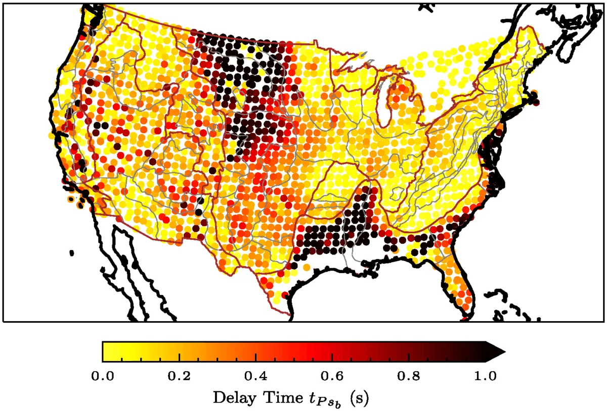
But in this study, the authors derive something called the time of phase of interest, or tPsb, from the data. To do so, they rely on receiver functions.
What’s a receiver function?
After a P-wave from a large earthquake travels through Earth and is measured at a distant seismic station (these are “teleseismic” events), additional waves arrive. Some of these later arrivals started off as P-waves, but were converted to S-waves as they bounced off a seismic discontinuity. Receiver functions — the time difference between the first P-wave and later arrivals — can reveal velocity contrasts at the discontinuity while also illuminating properties of the layers themselves.
Specifically, the authors used a precompiled set of seismic receiver functions from the NSF NGF data archive, from which they obtained radial receiver functions. However, gaps in this dataset exist, like in the southernmost part of the Gulf Coastal Plains and the interior California Central Valley — regions for which extremely thick sediments may complicate their receiver functions. In these cases, the authors re-computed the radial receiver functions using the same procedure as the precompiled dataset. In the end, the authors obtained measurements of the time of the phase of interest, tPsb, at 1,835 seismic stations.
The times show geographical patterns and spatial correlations with expected sedimentary basins. Large time delays should signal more sediment. For example, large time delays mark much of the Gulf Coast states, extending along the eastern seaboard next to the Appalachians. Large delays also appear in the Great Plains region. The Basin and Range of the western U.S. reflects alternating sediment-filled basins and high-standing ranges. In California, the Central Valley shows larger time delays than the mountains on either side — the Sierra Nevada and the Coast Ranges.
Calculating depth from time
Although receiver functions have been used to study structures within the crust and upper mantle of many regions, only recently have they been applied to the sediment that sheathes sections of the continents and seafloor. In this work, the authors rely on a single pick per receiver function, which is available even when the sediment layer is thin. This allows them to efficiently estimate continent-wide sediment thickness, and they do so in two ways.
The first method to estimate sediment thickness uses an empirical approach based on borehole-derived measurements of receiver functions from Australia. The equation requires tPsb and yields depth in meters. This helped the team determine whether the empirical relationship is transferable beyond Australia.
In the second method, the authors combine tPsb and with a seismic tomography model of the U.S. derived from Transportable Array data. The tomographic model provides a shear wave velocity model of the crust and upper mantle. The authors use the average velocity from the top five kilometers to represent sediment shear velocity. And so, with time from the receiver functions and velocity from the tomography, they calculated depth.
One map, two maps
By converting to depth in two ways, the authors assessed which method produced the best results. Though both maps show similar physiographic regional differences in thickness, the tomography-based method appeared to better approximate known sediment thickness.
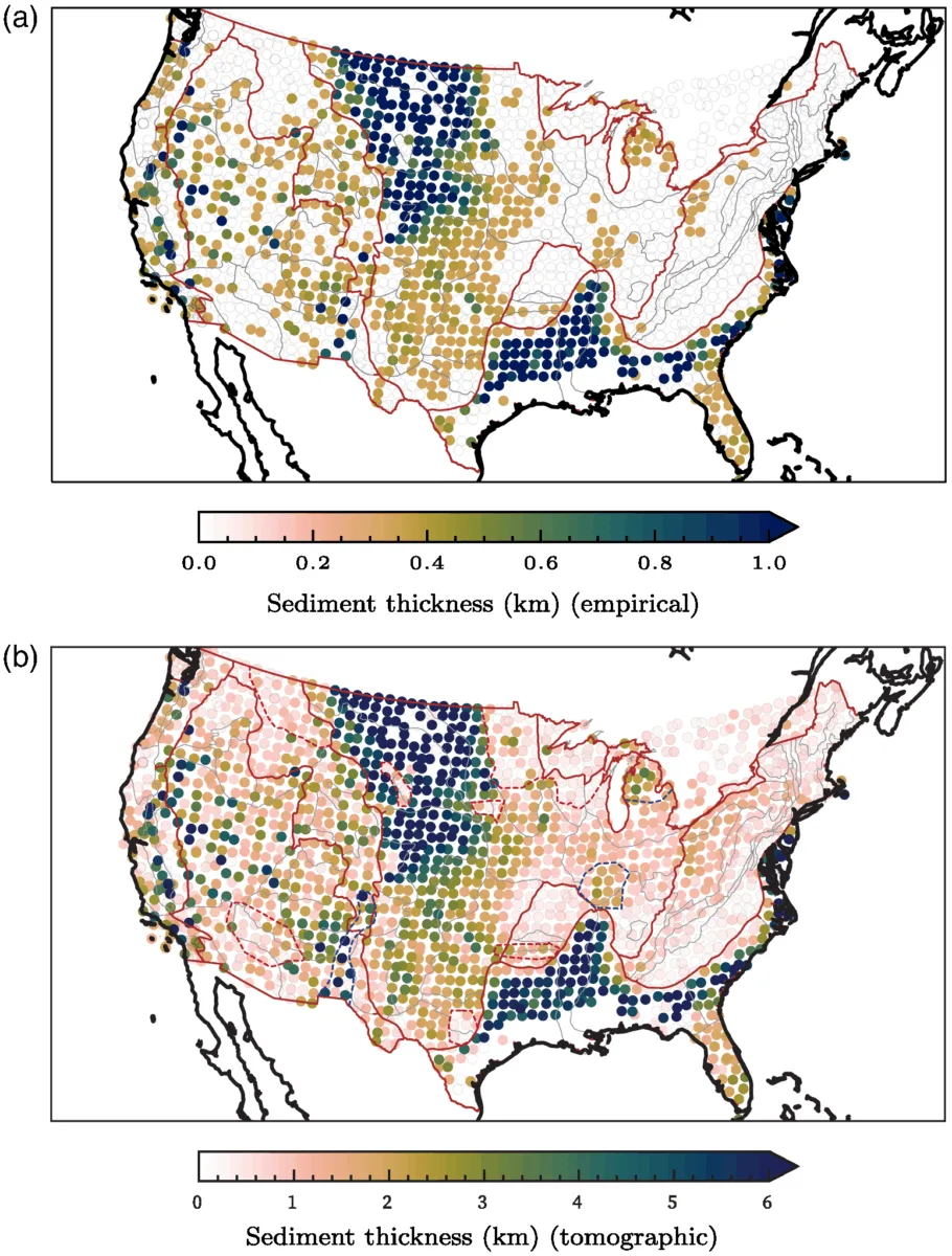
For example, in the Gulf Coastal Plain, the tomography-based method yielded thicknesses greater than six kilometers, whereas the empirical-based method yielded a thickness of less than two kilometers. This suggests that the empirical-based method, calibrated to Australia, may not be transferable to the U.S. The authors caution that the approaches presented in this paper — which begin with receiver functions — are suited to a study of large areas, whereas local studies of individual basins may require more sophisticated methods. Nevertheless, the authors write that the new map “can be used for future tomographic studies of the United States… as well as informing future estimates of national seismic hazard.”